
Figure
Founded Year
2022Stage
Series B | AliveTotal Raised
$854MValuation
$0000Last Raised
$675M | 7 mos agoMosaic Score The Mosaic Score is an algorithm that measures the overall financial health and market potential of private companies.
+29 points in the past 30 days
About Figure
Figure is an AI robotics company that focuses on developing general-purpose humanoid robots. Its main product, Figure 01, is a commercially viable autonomous humanoid robot designed to perform a variety of tasks across multiple industries, combining human-like dexterity with advanced artificial intelligence. Its humanoid robots are engineered to support sectors such as manufacturing, logistics, warehousing, and retail. It was founded in 2022 and is based in Sunnyvale, California.
Loading...
ESPs containing Figure
The ESP matrix leverages data and analyst insight to identify and rank leading companies in a given technology landscape.
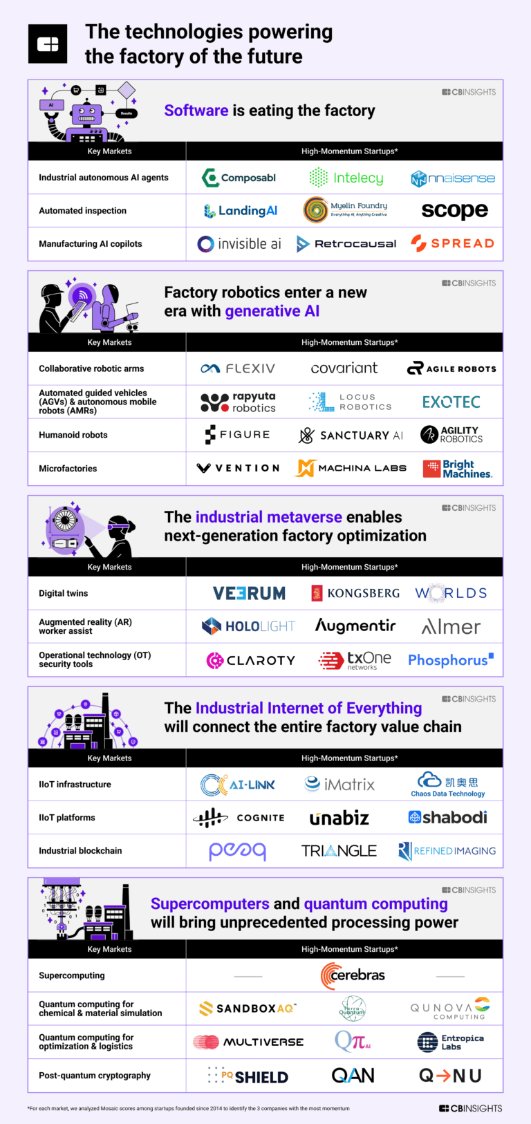
The industrial humanoid robot market specifically focuses on the development, manufacturing, and deployment of humanoid robots for use in industrial settings. Humanoid robots are designed to resemble the human body and are equipped with advanced sensors, actuators, and artificial intelligence capabilities. In industrial applications, humanoid robots are employed to perform tasks traditionally carr…
Figure named as Leader among 15 other companies, including Tesla, Boston Dynamics, and Agility Robotics.
Loading...
Research containing Figure
Get data-driven expert analysis from the CB Insights Intelligence Unit.
CB Insights Intelligence Analysts have mentioned Figure in 14 CB Insights research briefs, most recently on Aug 6, 2024.
May 31, 2024
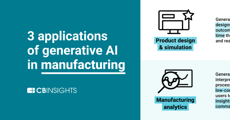
3 applications of generative AI in manufacturing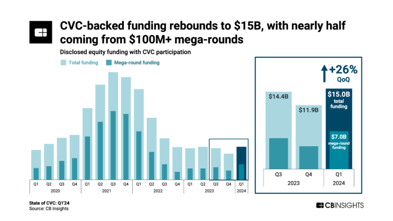
May 16, 2024 report
State of CVC Q1’24 Report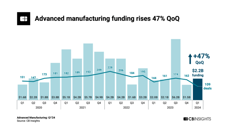
Apr 4, 2024 report
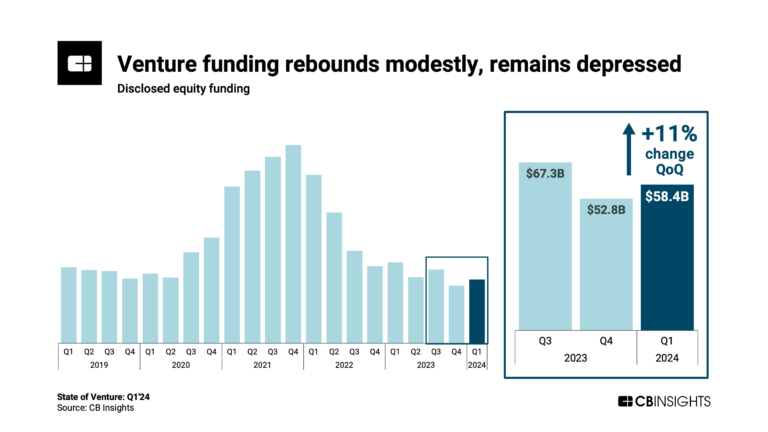
State of Venture Q1’24 ReportExpert Collections containing Figure
Expert Collections are analyst-curated lists that highlight the companies you need to know in the most important technology spaces.
Figure is included in 9 Expert Collections, including Artificial Intelligence.
Artificial Intelligence
14,769 items
Companies developing artificial intelligence solutions, including cross-industry applications, industry-specific products, and AI infrastructure solutions.
AI 100
100 items
Supply Chain & Logistics Tech
4,042 items
Companies offering technology-driven solutions that serve the supply chain & logistics space (e.g. shipping, inventory mgmt, last mile, trucking).
Advanced Manufacturing
6,353 items
Companies in the advanced manufacturing tech space, including companies focusing on technologies across R&D, mass production, or sustainability
AI 100 (2024)
100 items
Unicorns- Billion Dollar Startups
1,244 items
Latest Figure News
Sep 17, 2024
Abstract In computational molecular and materials science, determining equilibrium structures is the crucial first step for accurate subsequent property calculations. However, the recent discovery of millions of new crystals and super large twisted structures has challenged traditional computational methods, both ab initio and machine-learning-based, due to their computationally intensive iterative processes. To address these scalability issues, here we introduce DeepRelax, a deep generative model capable of performing geometric crystal structure relaxation rapidly and without iterations. DeepRelax learns the equilibrium structural distribution, enabling it to predict relaxed structures directly from their unrelaxed ones. The ability to perform structural relaxation at the millisecond level per structure, combined with the scalability of parallel processing, makes DeepRelax particularly useful for large-scale virtual screening. We demonstrate DeepRelax’s reliability and robustness by applying it to five diverse databases, including oxides, Materials Project, two-dimensional materials, van der Waals crystals, and crystals with point defects. DeepRelax consistently shows high accuracy and efficiency, validated by density functional theory calculations. Finally, we enhance its trustworthiness by integrating uncertainty quantification. This work significantly accelerates computational workflows, offering a robust and trustworthy machine-learning method for material discovery and advancing the application of AI for science. Introduction Atomic structure relaxation is usually the first step and foundation for further computational analysis of properties in computational chemistry, physics, materials science, and medicine. This includes applications such as chemical reactions on surfaces, complex defects in semiconductor heterostructures, and drug design. To date, computational relaxation algorithms have typically been achieved using iterative optimization, such as traditional ab initio methods, as shown in Fig. 1 a. For example, each iteration in density functional theory (DFT) calculations involves solving the Schrödinger equation to determine the electronic density distribution, from which the total energy of the system can be calculated. The forces on each atom, derived from differentiating this energy with respect to atomic positions, guide atomic movements to lower the system’s energy, typically using optimization algorithms. Despite its effectiveness, the high computational demands and poor scalability of DFT limit its applications across high-dimensional chemical and structural spaces 1 , such as the complex chemical reaction surfaces, doped semiconductor interfaces, or in the structural relaxation of the 2.2 million new crystals recently identified by DeepMind 2 . It is worth noting that the discovery of huge new materials has been significantly accelerated by high-throughput DFT calculations 3 , 4 , 5 , 6 and advanced machine learning (ML) algorithms 7 , 8 , 9 , 10 , which is promoting the development of more efficient relaxation algorithms. Fig. 1: An overview of ML methods for crystal structure relaxation. a Iterative ML methods that iteratively estimate energy and force to determine the equilibrium structure. b Illustration of our proposed DeepRelax method, which employs a periodicity-aware equivariant graph neural network (PaEGNN) to directly predict the relaxation quantities. Euclidean distance geometry (EDG) is then used to determine the final relaxed structure that satisfies the predicted relaxation quantities. ML has emerged as a promising alternative for predicting relaxed structures 1 , 11 , 12 , 13 , 14 , 15 , 16 , 17 , 18 . As conventional iterative optimization, iterative ML approaches 1 , 11 , 12 , 13 , 14 , 17 , 18 utilize surrogate ML models to approximate energy and forces at each iteration, as shown in Fig. 1 a, thereby circumventing the need to solve the computationally intensive Schrödinger equation. A typical example is the defect engineering in crystalline materials 19 , 20 , 21 . Mosquera-Lois et al. 13 and Jiang et al. 22 demonstrated that ML surrogate models could accelerate the optimization of crystals with defects. These ML models can retain DFT-level accuracy by training on extensive databases containing detailed information on structural relaxations, including energy, forces, and stress. However, there are two primary challenges in current iterative ML structural optimizers: training data limitations and non-scalability. Their training dataset must include full or partial intermediate steps of DFT relaxation. However, almost all publicized material databases, such as ICSD 23 and 2DMatPedia 6 , do not provide such structural information, potentially limiting the application of iterative ML methods. The other challenge is that the large-scale parallel processing capability of iterative ML methods is limited due to their step-by-step nature. To address this, Yoon et al. 16 developed a model called DOGSS, and Kim et al. 15 proposed a model named Cryslator. Both conceptually introduce direct ML approaches to predict the final relaxed structures from their unrelaxed counterparts. However, these approaches have only been validated on specific datasets or systems, and their universal applicability to diverse datasets or systems remains unproven. In this work, we introduce DeepRelax, a scalable, universal, and trustworthy deep generative model designed for direct structural relaxation. DeepRelax requires only the initial crystal structures to predict equilibrium structures in just a few hundred milliseconds on a single GPU. Furthermore, DeepRelax can efficiently handle multiple crystal structures in parallel by organizing them into mini-batches for simultaneous processing. This capability is especially advantageous in large-scale virtual screening, where rapid assessment of numerous unknown crystal configurations is essential. To demonstrate the reliability and robustness, we evaluate DeepRelax across five different datasets, including diverse 3D and 2D materials: the Materials Project (MP) 24 , X-Mn-O oxides 15 , 25 , the Computational 2D Materials Database (C2DB) 26 , 27 , 28 , layered van der Waals crystals, and 2D structures with point defects 19 , 21 . DeepRelax not only demonstrates superior performance compared to other direct ML methods but also exhibits competitive accuracy to the leading iterative ML model, M3GNet 11 , while being ~ 100 times faster in terms of speed. Moreover, we conduct DFT calculations to assess the energy of DeepRelax’s predicted structures, confirming our model’s ability to identify energetically favorable configurations. In addition, DeepRelax employs an uncertainty quantification method to assess the trustworthiness of the model. Finally, we would like to highlight that the aim of using DeepRelax is not to replace DFT relaxation but pre-relaxation, making the predicted structures very close to the DFT-relaxed configuration. Thus, the DFT method can rapidly complete the residual relaxation steps, significantly speeding up the traditional ab initio relaxation process, especially for complex structures. Results DeepRelax architecture DeepRelax emerges as a solution to the computational bottlenecks faced in DFT methods for crystal structure relaxation. Figure 1 b shows the workflow of DeepRelax, which takes an unrelaxed crystal structure as input and uses a periodicity-aware equivariant graph neural network (PaEGNN) to predict the relaxation quantities, including interatomic distances in the relaxed structure, displacements between the initial and relaxed structures, and the lattice matrix of the relaxed structure. DeepRelax then employs a numerical Euclidean distance geometry (EDG) solver to determine the relaxed structure that satisfies the predicted relaxation quantities. In addition, DeepRelax also quantifies bond-level uncertainty for each predicted interatomic distance and displacement. Aggregating these bond-level uncertainties allows for the computation of the system-level uncertainty, offering valuable insights into the trustworthiness of the model. A notable feature of PaEGNN, distinguishing it from previous graph neural networks (GNNs) 29 , 30 is the explicit differentiation of atoms in various translated cells to encode periodic boundary conditions (PBCs) using a unit cell offset encoding (UCOE). In addition, its design ensures equivariance, facilitating active exploration of crystal symmetries and thus providing a richer geometric representation of crystal structures. Benchmark on X-Mn-O dataset For our initial benchmarking, we utilize the X-Mn-O dataset, a hypothetical elemental substitution database previously employed for photoanode application studies 25 , 31 . This dataset derives from the MP database, featuring prototype ternary structures that undergo elemental substitution with X elements (Mg, Ca, Ba, and Sr). It consists of 28,579 data pairs, with each comprising an unrelaxed structure and its corresponding DFT-relaxed state. The dataset is divided into training (N = 22, 863), validation (N = 2, 857), and test (N = 2, 859) sets, adhering to an 8:1:1 ratio. As illustrated in Supplementary Fig. 1 , there are significant structural differences between the unrelaxed and DFT-relaxed structures within this dataset. We conduct a comparative analysis of DeepRelax against the state-of-the-art (SOTA) benchmark model, Cryslator 15 . In addition, we incorporate two types of equivariant graph neural networks-PAINN 29 and EGNN 32 -into our analysis (see Subsection 4.8 for the details). The choice of equivariant models is informed by recent reports highlighting their accuracy in direct coordinate prediction for structural analysis 32 , 33 , 34 . To ensure a fair comparison, we use the same training, validation, and testing sets across all models. As a baseline measure, we introduce a Dummy model, which simply returns the input initial structure as its output. This serves as a control reference in our evaluation process. To evaluate model performance, we use the mean absolute error (MAE) of Cartesian coordinates, bond lengths, lattice matrix, and cell volume to measure the consistency between predicted and DFT-relaxed structures. In addition, we calculate the match rate–a measure of how closely predicted relaxed structures align with their ground truth counterparts within a defined tolerance, as determined by Pymatgen 3 . Detailed descriptions of these metrics are provided in Subsection 4.10. Table 1 presents the comparative results, showing that DeepRelax greatly outperforms other baselines. Notably, DeepRelax shows a remarkable improvement in prediction accuracy over the Dummy model, with enhancements of 63.06%, 68.30%, 71.49%, 89.63%, and 30.71% across coordinates, bond lengths, lattice, cell volumes, and match rate, respectively. Moreover, DeepRelax surpasses the previous SOTA model, Cryslator, by 8.66% in coordinate prediction, and 45.16% in cell volume estimation. Figure 2 a shows the distribution of MAE for coordinates, lattice matrix, and cell volumes as predicted by the Dummy model and DeepRelax. DeepRelax demonstrates a notable leftward skewness in its distribution, signifying a tendency to predict structures that closely approach the DFT-relaxed state. To visualize the performance of DeepRelax, we take two typical structures, Sr4Mn2O6 and Ba1Mn4O8, from the X-Mn-O database (see Fig. 3 ), and relax them using DeepRelax. As can be seen, the DeepRelax-predicted structures are highly consistent with the DFT-relaxed ones. The results demonstrate close agreement with DFT-relaxed structures. More DFT validations are in Subsection 2.7. Table 1 Comparative results of DeepRelax and baseline models on the X-Mn-O dataset, evaluated based on MAE of coordinates (Å), bond length (Å), lattice (Å), cell volume (Å3), and match rate (%) between the predicted and DFT-relaxed structures Fig. 2: Distribution of MAE for predicted structures by the Dummy model and DeepRelax. a X-Mn-O dataset, (b) MP dataset, and (c) C2DB dataset. Each subfigure, from left to right, displays the MAE for coordinates (Å), lattice matrices (Å), and cell volumes (Å3), respectively. Source data are provided in this paper. Fig. 3: Visualization of two crystal structures relaxed by DeepRelax. a Sr4Mn2O6 and (b) Ba1Mn4O8, where a, b, and c are lattice constants in angstroms (Å), and α, β, and γ are angles in degrees (∘). The results demonstrate close agreement between DeepRelax-predicted structures and DFT-relaxed structures. Benchmark on Materials Project To demonstrate DeepRelax’s universal applicability across various elements of the periodic table and diverse crystal types, we conduct further evaluations using the Materials Project dataset 11 . This dataset spans 89 elements and comprises 187,687 snapshots from 62,783 compounds captured during their structural relaxation processes. By excluding compounds missing either initial or DFT-relaxed structures, we refined the dataset to 62,724 pairs. Each pair consists of an initial and a corresponding DFT-relaxed structure, providing a comprehensive basis for assessing the performance of DeepRelax. This dataset is then split into training, validation, and test data in the ratio of 90%, 5%, and 5%, respectively. As illustrated in Supplementary Fig. 1 , the structural differences for each pair tend toward an MAE of zero, indicating that many initial structures are closely aligned with their DFT-relaxed counterparts. Training a direct ML model for datasets with varied compositions poses significant challenges, as evidenced in Cryslator 15 . This model shows reduced prediction performance when trained on the diverse MP database. Despite these challenges, DeepRelax demonstrates its robustness and universality. As indicated in Table 2 , DeepRelax significantly surpasses the three baseline models in coordinate prediction, highlighting its effectiveness even in diverse and complex datasets. Figure 2 b shows the MAE distribution for predicted structures compared to the DFT-relaxed ones for the MP dataset, which is less significant compared to the results for the X-Mn-O dataset shown in Fig. 2 a. This is because many initial structures closely resemble their DFT-relaxed structures in the MP database as evidenced by Supplementary Fig. 1 . Consequently, the MP dataset presents a more complex learning challenge for structural relaxation models. Table 2 Comparison of results between the proposed DeepRelax and other models on the MP dataset. The performances are evaluated by the MAE of coordinates (Å), bond length (Å), lattice (Å), and cell volume (Å3) between the predicted and DFT-relaxed structures Transfer learning on 2D materials database Given that most materials databases do not provide the energy and force information of unrelaxed structures, it is difficult for conventional iterative ML models to transfer the trained model from Materials Project to other materials databases. This difficulty arises because transfer learning typically depends on the availability of energy and force information to fine-tune the model. DeepRelax, with its direct structural prediction feature, is more compatible with transfer learning, making it a flexible tool even when only structural data are available. To demonstrate the reliable application of DeepRelax, we extend the application of DeepRelax, initially pre-trained on 3D materials from the MP dataset, to 2D materials through transfer learning. We take the C2DB dataset 26 , 27 , 28 as an example, which covers 62 elements and comprises 11,581 pairs of 2D crystal structures, each consisting of an initial and a DFT-relaxed structure. The dataset is divided into training, validation, and testing subsets, maintaining a ratio of 6:2:2. The structural differences for each pair in this dataset fall within the range observed for the X-Mn-O and MP datasets, as shown in Supplementary Fig. 1 . In this application, DeepRelax trained via transfer learning is denoted as DeepRelaxT to differentiate it from DeepRelax. Table 3 illustrates our key findings: Firstly, both DeepRelax and DeepRelaxT outperform the other three baselines in the C2DB dataset, proving the applicability of our direct ML model to 2D materials. Figure 2 c presents the MAE distribution for predicted structures by the Dummy model and DeepRelax on the C2DB dataset. These results suggest a modest improvement over the Dummy model. Notably, this improvement surpasses those observed for the MP dataset, as depicted in Fig. 2 b. Secondly, DeepRelaxT demonstrates notable improvements over DeepRelax, with enhancements of 5.61% in coordinates, 38.43% in bond length, 3.53% in lattice, and 5.81% in cell volume in terms of MAE. Finally, DeepRelaxT shows a faster convergence rate than DeepRelax, as detailed in Supplementary Fig. 2 . These results underline the benefits of large-scale pretraining and the efficacy of transfer learning. Table 3 Comparison of results among DeepRelax, DeepRelaxT (transfer learning version), and other models on the C2DB dataset. The performances are evaluated by the MAE of coordinates (Å), bond length (Å), lattice (Å), and cell volume (Å3) between the predicted and DFT-relaxed structures Application in layered vdW crystals Layered vdW crystals are of significant interest in the field of materials science and nanotechnology because of their unique tunable structures, such as twisting and sliding configurations 35 . One notable characteristic of these crystals is that the weak inter-layer vdW force may significantly change upon full relaxation, while the strong intra-layer chemical bonds undergo relatively small changes. To demonstrate the reliable performance of our DeepRelax model on this type of crystal, we performed DFT relaxation of 58 layered vdW crystals covering 29 elements using van der Waals corrections, parameterized within the DFT-D3 Grimme method. Given the small sample size, we employ transfer learning, utilizing a model pre-trained on the Materials Project dataset. Supplementary. Table 1 shows the inter-layer distances for the unrelaxed, DFT-D3-relaxed, and DeepRelax-predicted structures of six vdW layered crystals. The inter-layer distances of the predicted structures closely match those of the relaxed structures, highlighting the effectiveness of transferred DeepRelax on layered vdW crystals. Furthermore, an analysis of the MAE in bond length for representative bonding pairs, detailed in Supplementary Table 2 , further demonstrates DeepRelax’s precision in predicting structural changes in layered vdW crystals. Application in crystals with defects Most crystals have intrinsic defects. To demonstrate the robustness of DeepRelax to crystal structures with neutral point defects, we employ MoS2 structures with a low defect concentration, including 5933 different defect configurations within an 8 × 8 supercell, as cataloged by Huang et al. 21 , to evaluate DeepRelax. Supplementary Fig. 3 demonstrates a notably lower MAE in both atom coordinates and bond lengths for DeepRelax compared to the Dummy model, thereby underscoring DeepRelax’s robustness and efficacy in defect structure calculations, which is further validated by DFT calculations in the next chapter. DFT validations Usually, the initial crystal structure may deviate from or be close to the final relaxed structure. To demonstrate the efficacy and robustness of DeepRelax, we perform DFT validations on two types of initial structures: those from the X-Mn-O dataset, which exhibit large deviations from the DFT-relaxed state, and those from the MP dataset, which are generally closer to their DFT-relaxed structures, as illustrated in Supplementary Fig. 1 . The detailed settings for the DFT calculations are provided in Subsection 4.9. In the first experiment, we evaluated our model’s predictive capability under challenging conditions using the X-Mn-O dataset. We filtered out unrelaxed structures from the X-Mn-O test set that are structurally similar to their DFT-relaxed counterparts using Pymatgen’s “Structure_matcher" function. From the remaining test set (N = 1007), we randomly selected 100 samples. Figure 4 a shows the deviation distribution for the selected unrelaxed structures, which closely aligns with that of the complete test set, thus confirming the representativeness of the selected subset. Subsequently, we employed DeepRelax to predict the relaxed structures for these samples. Figure 4 b shows box plots of the energy distributions for the unrelaxed, DFT-relaxed, and DeepRelax-predicted structures. The energy distributions of the DeepRelax-predicted and DFT-relaxed structures show similar medians and interquartile ranges, validating the model’s accuracy in predicting energetically favorable structures. The MAE in energy is significantly reduced by an order of magnitude from 32.51 to 5.97. Fig. 4: DFT validations. a Distributions of deviations for 100 random samples from the X-Mn-O dataset, measured using MAE in coordinates (Å) between the unrelaxed and DFT-relaxed structures. b Energy distribution for the three types of structures among the 100 random samples from the X-Mn-O dataset. The boxplots show the median (black line inside the box), interquartile range (box), and whiskers extending to 1.5 times the interquartile range, with outliers plotted as individual points. c Distribution of deviations for 100 random samples from the Materials Project dataset with relatively rational initial structures. d Energy distribution for the three types of structures among the 100 random samples from the Materials Project dataset. e Distributions of deviations for 20 random samples from the 2D materials defect dataset. f The number of DFT ionic steps required to complete DFT structure relaxation, starting from the initial unrelaxed structures and the DeepRelax-predicted structures, respectively. The samples are sorted based on the number of ionic steps required by the unrelaxed structures for better observation. Source data are provided in this paper. In the second experiment, we tested whether DeepRelax remains effective with structures starting from a relatively rational initial unrelaxed state using the Materials Project dataset. Here, we again randomly selected 100 samples from the test set. Figure 4 c shows the deviation distribution for these samples. The energies of the unrelaxed, DFT-relaxed, and DeepRelax-predicted structures were calculated using DFT. Figure 4 d shows that the predicted structures feature an energy distribution nearly identical to that of the DFT-relaxed structures, demonstrating the model’s effectiveness in handling relatively rational initial unrelaxed structures. Besides the energy indicator, we further demonstrated our model’s effectiveness using the number of residual optimizing (ionic) steps required for DFT relaxation. Specifically, we randomly selected 20 structures from the test set of the point-defect dataset, with their deviation distribution as shown in Fig. 4 e. We then conducted DFT calculations starting from the unrelaxed and DeepRelax-predicted structures, respectively. As shown in Fig. 4 f, starting DFT relaxation from the DeepRelax-predicted structures significantly reduces the number of required ionic steps, which is also robust. Analysis of uncertainty A critical challenge in integrating artificial intelligence (AI) into material discovery is establishing trustworthy AI models. Current deep learning models typically offer accurate predictions only within the chemical space covered by their training datasets, known as the applicability domain 36 . Predictions for samples outside this domain can be questionable. Thus, uncertainty quantification has become critical for AI models by quantifying prediction confidence levels, thereby aiding researchers in decision-making and experimental planning. To validate the efficacy of our proposed uncertainty quantification in reflecting the confidence level of model predictions, we compute Spearman’s rank correlation coefficient between the total predicted distance error and its associated system-level uncertainty. Figure 5 a–c shows the hexagonal binning plots of system-level uncertainty against total distance MAE for the X-Mn-O, MP, and C2DB datasets, respectively. Correlation coefficients of 0.95, 0.83, and 0.88 for these datasets demonstrate a strong correlation between predicted error and predicted system-level uncertainty. Figure 5 d, e presents the bond-level uncertainty visualization for two predicted structures, illustrating the correlation between predicted bond length error and associated bond-level uncertainty. These results indicate that the model’s predicted uncertainty is a good indicator of the predicted structure’s accuracy. Fig. 5: Uncertainty quantification. Hexagonal binning plots comparing system-level uncertainty with distance MAE (Å) for the (a) X-Mn-O, (b) MP, and (c) C2DB datasets. d, e illustrate the bond-level uncertainty for each predicted pairwise distance in Sr2Mn2O4 and Mg1Mn1O3, respectively, demonstrating the correlation between distance prediction errors and their associated bond-level uncertainties. Source data are provided in this paper. Ablation study DeepRelax’s technical contributions are twofold: it utilizes UCOE for handling PBCs explicitly, and it employs a method for estimating bond-level data uncertainty to encourage the model to capture a more comprehensive representation of the underlying data distribution. To validate the effectiveness of these two strategies, we introduce three additional baseline models for comparison: Vanilla: Excludes both UCOE and data uncertainty estimation. DeepRelax (UCOE): Integrates UCOE but omits data uncertainty estimation. DeepRelax (BLDU): Implements bond-level data uncertainty estimation but not UCOE. Table 4 demonstrates that DeepRelax (UCOE) attains a significant performance enhancement over the Vanilla model, suggesting the UCOE contributes greatly to model performance. On the other hand, DeepRelax (BLDU) shows a more modest improvement, which indicates the added value of data uncertainty estimation. Overall, DeepRelax shows a 25.16% improvement in coordinate MAE and a 20.00% advancement in bond length MAE over the Vanilla model. These comparative results underscore the combined effectiveness of UCOE and data uncertainty estimation in our final DeepRelax model. Table 4 Ablation study to investigate the impact of unit cell offset encoding (UCOE) and bond-level data uncertainty (BLDU) estimation on model performance. The performances are evaluated by the MAE of coordinates (Å), bond length (Å), lattice (Å), and cell volume (Å3) between the predicted and DFT-relaxed structures To actively explore the crystal symmetry, each node \({v}_{i}\in {{\mathcal{V}}}\) is assigned both a scalar feature \({{{\boldsymbol{x}}}}_{i}\in {{\mathbb{R}}}^{F}\) and a vector feature \({\overrightarrow{{{\boldsymbol{x}}}}}_{i}\in {{\mathbb{R}}}^{F\times 3}\), i.e., retaining F scalars and F vectors for each node. These features are updated in a way that preserves symmetry during training. The scalar feature \({{{\boldsymbol{x}}}}_{i}^{(0)}\) is initialized as an embedding dependent on the atomic number, \(E({z}_{i})\in {{\mathbb{R}}}^{F}\), where zi is the atomic number, and E is an embedding layer mapping zi to a F-dimensional feature vector. This embedding is similar to the one-hot vector but is trainable. The vector feature is initially set to zero, \({\overrightarrow{{{\boldsymbol{x}}}}}_{i}^{(0)}=\overrightarrow{{{\mathbf{0}}}}\in {{\mathbb{R}}}^{F\times 3}\). In addition, we define \({\overrightarrow{{{\boldsymbol{r}}}}}_{ij}={\overrightarrow{{{\boldsymbol{r}}}}}_{j}-{\overrightarrow{{{\boldsymbol{r}}}}}_{i}\) as the vector from node vi to vj. Periodicity-aware equivariant graph neural network PaEGNN iteratively updates node representations in two phases: message passing and updating. These phases are illustrated in Fig. 6 b and further detailed in Fig. 6 c–e. During message passing, nodes receive information from neighboring nodes, expanding their accessible radius. In the updating phase, PaEGNN utilizes the node’s internal messages (composed of F scalars and F vectors) to update its features. To prevent over-smoothing 58 , 59 , skip connections are added to each layer. In subsequent sections, we define the norm ∥ ⋅ ∥ and dot product 〈 ⋅ , ⋅ 〉 as operations along the spatial dimension, while concatenation ⊕ and the element-wise product ∘ are performed along the feature dimension. Unit cell offset encoding A notable feature of PaEGNN, distinguishing it from previous models 29 , 30 , is the explicit differentiation of atoms in various translated unit cells to encode PBCs. To achieve this, we define the set \({{\mathcal{C}}}=\{-2,-1,\,0,\,1,\,2\}\). We then use this set to generate translated unit cells with offsets \(({k}_{1},\,{k}_{2},\,{k}_{3})\in {{\mathcal{C}}}\times {{\mathcal{C}}}\times {{\mathcal{C}}}\). The translated unit cells, resulting from the offsets \(({k}_{1},\,{k}_{2},\,{k}_{3})\in {{\mathcal{C}}}\times {{\mathcal{C}}}\times {{\mathcal{C}}}\), are generally sufficient to encompass all atoms within a 6Å cutoff distance. We use \({({k}_{1},\,{k}_{2},\,{k}_{3})}_{ij}\) to denote the unit cell offset from node vi to node vj, where node vj is located in a unit cell translated by \({k}_{1}{\overrightarrow{{{\boldsymbol{l}}}}}_{1}+{k}_{2}{\overrightarrow{{{\boldsymbol{l}}}}}_{2}+{k}_{3}{\overrightarrow{{{\boldsymbol{l}}}}}_{3}\) relative to node vi. Let Kij = (k1 + 2) + (k2 + 2)5 + (k3 + 2)25 be a positive integer that uniquely indexes the unit cell offset, the sinusoidal positional encoding 60 for Kij is computed as: $$p({K}_{ij},\,f)=\left\{\begin{array}{lr}\sin ({K}_{ij}/1000{0}^{\,f/F}),\hfill &\,{{\rm{if}}}\,\,f\in \{0,2,4,\ldots,F-2\}\\ \cos ({K}_{ij}/1000{0}^{\,(f-1)/F}),&\,{{\rm{if}}}\,\,f\in \{1,3,5,\ldots,F-1\}\end{array}\right.$$ (2) The full positional encoding vector is then $${{\boldsymbol{p}}}({K}_{ij})=\left(p({K}_{ij},\,0),\,p({K}_{ij},\,1),\ldots,\,p({K}_{ij},\,F-1)\right)\in {{\mathbb{R}}}^{F}$$ (3) The unit cell offset encoding p(Kij) explicitly encodes the relative position of the unit cells in which the two nodes, vi and vj, are located. This encoding enables the GNN to explicitly recognize the periodic structure, thereby enhancing predictive performance. Message passing phase During this phase, a node vi aggregates messages from neighboring scalars \({{{\boldsymbol{x}}}}_{j}^{(t)}\) and vectors \({\overrightarrow{{{\boldsymbol{x}}}}}_{j}^{(t)}\), forming intermediate scalar and vector variables mi and \({\overrightarrow{{{\boldsymbol{m}}}}}_{i}\) as follows: $${{{\boldsymbol{m}}}}_{i}=\sum\limits_{{v}_{j}\in {{\mathcal{N}}}({v}_{i})}({{{\boldsymbol{W}}}}_{h}{{{\boldsymbol{x}}}}_{j}^{(t)})\,{\circ} \,\,\,{\gamma }_{h}\left(\lambda (\parallel {\overrightarrow{{{\boldsymbol{r}}}}}_{ji}\parallel )\oplus {{\boldsymbol{p}}}({K}_{ji})\right)$$ (4) $$\begin{array}{rc}{\overrightarrow{{{\boldsymbol{m}}}}}_{i}=\sum\limits_{{v}_{j}\in {{\mathcal{N}}}({v}_{i})}&({{{\boldsymbol{W}}}}_{u}{{{\boldsymbol{x}}}}_{j}^{(t)})\,{\circ} \,\,\, {\gamma }_{u}\left(\lambda (\parallel {\overrightarrow{{{\boldsymbol{r}}}}}_{ji}\parallel )\oplus {{\boldsymbol{p}}}({K}_{ji})\right)\,{\circ} \,\,\, {\overrightarrow{{{\boldsymbol{x}}}}}_{j}^{(t)}\\ &+({{{\boldsymbol{W}}}}_{v}{{{\boldsymbol{x}}}}_{j}^{(t)})\,{\circ} \,\,\,{\gamma }_{v}\left(\lambda (\parallel {\overrightarrow{{{\boldsymbol{r}}}}}_{ji}\parallel )\oplus {{\boldsymbol{p}}}({K}_{ji})\right)\,{\circ} \,\,\, \frac{{\overrightarrow{{{\boldsymbol{r}}}}}_{ji}}{\parallel {\overrightarrow{{{\boldsymbol{r}}}}}_{ji}\parallel }\end{array}$$ (5) Here, ⊕ denotes concatenation, \({{\mathcal{N}}}({v}_{i})\) represents the neighboring nodes of vi, \({{{\boldsymbol{W}}}}_{h},{{{\boldsymbol{W}}}}_{u},{{{\boldsymbol{W}}}}_{v}\in {{\mathbb{R}}}^{F\times F}\) are trainable weight matrices, λ is a set of Gaussian radial basis functions (RBF) 46 that are used to expand bond distances, and γh, γu, and γv are a linear projection mapping the concatenated feature back to F-dimensional space. Message updating phase The updating phase concentrates on integrating the F scalars and F vectors within mi and \({\overrightarrow{{{\boldsymbol{m}}}}}_{i}\) to generate updated scalar \({{{\boldsymbol{x}}}}_{i}^{(t+1)}\) and vector \({\overrightarrow{{{\boldsymbol{x}}}}}_{i}^{(t+1)}\): $${{{\boldsymbol{x}}}}_{i}^{(t+1)}={{{\boldsymbol{W}}}}_{s1}({{{\boldsymbol{m}}}}_{i}\oplus \parallel {{\boldsymbol{U}}}{\overrightarrow{{{\boldsymbol{m}}}}}_{i}\parallel )+{{{\boldsymbol{W}}}}_{s2}({{{\boldsymbol{m}}}}_{i}\oplus \parallel {{\boldsymbol{U}}}{\overrightarrow{{{\boldsymbol{m}}}}}_{i}\parallel )\langle {{\boldsymbol{V}}}{\overrightarrow{{{\boldsymbol{m}}}}}_{i},{{\boldsymbol{U}}}{\overrightarrow{{{\boldsymbol{m}}}}}_{i}\rangle$$ (6) $${\overrightarrow{{{\boldsymbol{x}}}}}_{i}^{(t+1)}={{{\boldsymbol{W}}}}_{v}({{{\boldsymbol{m}}}}_{i}\oplus \parallel {{\boldsymbol{U}}}{\overrightarrow{{{\boldsymbol{m}}}}}_{i}\parallel )\,{\circ} \,\,\, ({{\boldsymbol{V}}}{\overrightarrow{{{\boldsymbol{m}}}}}_{i})$$ (7) where \({{{\boldsymbol{W}}}}_{s1},\,{{{\boldsymbol{W}}}}_{s2},\,{{{\boldsymbol{W}}}}_{v}\in {{\mathbb{R}}}^{F\times 2F}\) and \({{\boldsymbol{U}}},{{\boldsymbol{V}}}\in {{\mathbb{R}}}^{F\times F}\). Predicting relaxation quantities Assuming PaEGNN comprises T layers, we define the bond feature \({{{\boldsymbol{h}}}}_{ij}=\gamma \left(\lambda (\parallel {\overrightarrow{{{\boldsymbol{r}}}}}_{ij}\parallel )\oplus {{\boldsymbol{p}}}({k}_{1},\,{k}_{2},\,{k}_{3})\right)\), where γ is a linear projection mapping the concatenated feature back to F-dimensional space. The prediction of a pairwise distance \({\hat{d}}_{ij}\) for the edge \({e}_{ij,({k}_{1},\,{k}_{2},\,{k}_{3})}\) is formulated as: $${\hat{d}}_{ij}=| \, {f}_{d}({{{\boldsymbol{W}}}}_{d}{{{\boldsymbol{x}}}}_{i}^{(T)}\oplus {{{\boldsymbol{W}}}}_{d}{{{\boldsymbol{x}}}}_{j}^{(T)}\oplus {{{\boldsymbol{h}}}}_{ij})|$$ (8) where \({{{\boldsymbol{W}}}}_{d}\in {{\mathbb{R}}}^{F\times F}\) is a learnable matrix and \({f}_{d}:{{\mathbb{R}}}^{3F}\to {\mathbb{R}}\) is a linear map. Using Eqn. ( 8 ), we can predict both the interatomic distances in the relaxed structure and the displacements between the initial and relaxed structures. In addition, DeepRelax predicts the lattice matrix of the relaxed structure as follows: $$\hat{{{\boldsymbol{L}}}}={r}_{L}\left({f}_{L}\left({{{\boldsymbol{W}}}}_{l}\left({\overrightarrow{{{\boldsymbol{l}}}}}_{1}\oplus {\overrightarrow{{{\boldsymbol{l}}}}}_{2}\oplus {\overrightarrow{{{\boldsymbol{l}}}}}_{3}\right)\oplus \left(\sum\limits_{{v}_{i}\in {{\mathcal{G}}}}{{{\boldsymbol{W}}}}_{x}{{{\boldsymbol{x}}}}_{i}\right)\right)\right)$$ (9) Here, \({{{\boldsymbol{W}}}}_{x}\in {{\mathbb{R}}}^{F\times F}\), \({{{\boldsymbol{W}}}}_{l}\in {{\mathbb{R}}}^{9\times F}\), and \({f}_{L}:{{\mathbb{R}}}^{2F}\to {{\mathbb{R}}}^{9}\) is a linear mapping yielding a 9-dimensional vector Lv. The operation rL reshapes Lv into a 3 × 3 matrix \(\hat{{{\boldsymbol{L}}}}\) to reflect the lattice vectors. Uncertainty-aware loss function In real scenarios, each predicted distance is subject to inherent noise (e.g., measurement errors or human labeling errors). To capture this uncertainty, we can model the pairwise distances as random variables following a Laplace distribution, i.e., \({d}_{ij} \sim \,{\mbox{Laplace}}\,({\hat{d}}_{ij},{\hat{b}}_{ij})\). Here, \({\hat{d}}_{ij}\) and \({\hat{b}}_{ij}\) are the location parameter and scale parameter, respectively. In our application, \({\hat{d}}_{ij}\) represents the predicted distance and \({\hat{b}}_{ij}\) represents the associated bond-level data uncertainty. The scale parameter \({\hat{b}}_{ij}\) is predicted as follows: $${\hat{b}}_{ij}={f}_{b}({{{\boldsymbol{W}}}}_{b}{{{\boldsymbol{x}}}}_{i}^{(T)}\oplus {{{\boldsymbol{W}}}}_{b}{{{\boldsymbol{x}}}}_{j}^{(T)}\oplus {{{\boldsymbol{h}}}}_{ij})$$ (10) where \({{{\boldsymbol{W}}}}_{b}\in {{\mathbb{R}}}^{F\times F}\) is a learnable matrix, and \({f}_{b}:{{\mathbb{R}}}^{3F}\to {\mathbb{R}}\) is a linear map. To train DeepRelax such that its output follows the assumed Laplace distribution, we propose an uncertainty-aware loss \({{{\mathcal{L}}}}_{u}\), which comprises interatomic distance loss \({{{\mathcal{L}}}}_{i}\) and displacement loss \({{{\mathcal{L}}}}_{d}\): $${{{\mathcal{L}}}}_{i}=\sum\limits_{{e}_{ij,({k}_{1},\,{k}_{2},\,{k}_{3})}\in {{\mathcal{E}}}}\log (2{\hat{b}}_{ij})+\frac{| {d}_{ij}-{\hat{d}}_{ij}| }{{\hat{b}}_{ij}}$$ (11) $${{{\mathcal{L}}}}_{d}=\sum\limits_{{e}_{ij,\,(0,\,0,\,0)}\in {{\mathcal{E}}}}\log (2{\hat{b}}_{ij})+\frac{| {d}_{ij}-{\hat{d}}_{ij}| }{{\hat{b}}_{ij}}$$ (12) (13) In these expressions, dij represents the ground truth distance. The edges \({e}_{ij,({k}_{1},\,{k}_{2},\,{k}_{3})}\in {{\mathcal{E}}}\) pertain to interatomic distance predictions, whereas \({e}_{ij,\,(0,\,0,\,0)}\in {{\mathcal{E}}}\) denotes edges used for displacement predictions within the unit cell, discounting PBCs. In essence, \({{{\mathcal{L}}}}_{i}\) and \({{{\mathcal{L}}}}_{d}\) represents the negative log-likelihood of the Laplace distribution, thereby capturing the data uncertainty. Consequently, a larger \({\hat{b}}_{ij}\) indicates greater bond-level data uncertainty in the prediction, and vice versa. The total loss \({{\mathcal{L}}}\) is consist of \({{{\mathcal{L}}}}_{u}\) and a lattice loss \({{{\mathcal{L}}}}_{l}\): $${{{\mathcal{L}}}}_{l}=\sum | \hat{{{\boldsymbol{L}}}}-{{\boldsymbol{L}}}|$$ (14) Numerical Euclidean distance geometry solver We propose a numerical EDG solver to determine the relaxed structure that aligns with the predicted relaxation quantities. Specifically, for a given graph \({{\mathcal{G}}}=({{\mathcal{V}}},{{\mathcal{E}}},d)\) and a dimension K, the EDG problem 61 , 62 , 63 seeks a realization-specifically, a coordinate matrix \(\hat{{{\boldsymbol{R}}}}\in {{\mathbb{R}}}^{N\times K}:{{\mathcal{V}}}\to {{\mathbb{R}}}^{K}\) in K-dimensional space that satisfies the distance constraint d as follows: $$\forall (u,\,v)\in {{\mathcal{E}}},\parallel \hat{{{\boldsymbol{R}}}}(u)-\hat{{{\boldsymbol{R}}}}(v)\parallel={d}_{uv}$$ (16) For simplicity in notation, \(\hat{{{\boldsymbol{R}}}}(u)\) and \(\hat{{{\boldsymbol{R}}}}(v)\) are typically written as \({\hat{{{\boldsymbol{R}}}}}_{u}\) and \({\hat{{{\boldsymbol{R}}}}}_{v}\). We reformulate the conventional EDG problem into a global optimization task: $${{{\mathcal{L}}}}_{g}=\sum\limits_{(u,v)\in {{\mathcal{E}}}}| \parallel {\hat{{{\boldsymbol{R}}}}}_{u}-{\hat{{{\boldsymbol{R}}}}}_{v}\parallel -{d}_{uv}|$$ (17) This is a non-convex optimization problem, and minimizing \({{{\mathcal{L}}}}_{g}\) gives an approximation solution of \(\hat{{{\boldsymbol{R}}}}\). In our specific application, we aim to find a coordinate matrix \(\hat{{{\boldsymbol{R}}}}\in {{\mathbb{R}}}^{N\times 3}\) for a system of N atoms in three-dimensional space, meeting the constraints imposed by \({\hat{d}}_{ij}\), \({\hat{b}}_{ij}\), and \(\hat{{{\boldsymbol{L}}}}\). Specifically, we first define an upper bound and a lower bound using \({\hat{d}}_{ij}\), \({\hat{b}}_{ij}\) as following: $${\hat{d}}_{ij}^{u}={\hat{d}}_{ij}+\exp ({\hat{b}}_{ij})$$ (18) (19) Subsequently, we propose minimizing a bounded Euclidean distance (BED) loss: $$\begin{array}{rc}{{{\mathcal{L}}}}_{g}=&\sum\limits_{\begin{array}{c}{e}_{ij,\, ({k}_{1},\,{k}_{2},\,{k}_{3})}\in {{\mathcal{E}}}\\ {e}_{ij,(0,0,0)}\in {{\mathcal{E}}}\end{array}}\max (0,\parallel {\hat{{{\boldsymbol{R}}}}}_{u}-{\hat{{{\boldsymbol{R}}}}}_{v}\parallel -{\hat{d}}_{ij}^{u})\\ &+\sum\limits_{\begin{array}{c}{e}_{ij,({k}_{1},{k}_{2},{k}_{3})}\in {{\mathcal{E}}}\\ {e}_{ij,(0,0,0)}\in {{\mathcal{E}}}\end{array}}\max (0,\, {{\hat{d}^{l}_{ij}}}-\parallel {\hat{{{\boldsymbol{R}}}}}_{u}-{\hat{{{\boldsymbol{R}}}}}_{v}\parallel )\end{array}$$ (20) For each edge \({e}_{ij,({k}_{1},{k}_{2},{k}_{3})}\), the location of node vj is dictated by \({k}_{1}{\hat{{{\boldsymbol{l}}}}}_{1}+{k}_{2}{\hat{{{\boldsymbol{l}}}}}_{2}+{k}_{3}{\hat{{{\boldsymbol{l}}}}}_{3}\), where \({\hat{{{\boldsymbol{l}}}}}_{1}\), \({\hat{{{\boldsymbol{l}}}}}_{2}\), \({\hat{{{\boldsymbol{l}}}}}_{3}\) are predicted lattice vectors. The BED loss only penalizes coordinate pairs whose distances fall outside the lower and upper bounds, thus mitigating the impact of less accurate predictions. In our work, we use Adam optimizer to minimize \({{{\mathcal{L}}}}_{g}\). Uncertainty quantification We initially quantify bond-level uncertainties and subsequently aggregate these to determine the system-level uncertainty of the predicted structure. The bond-level uncertainty can be further decomposed into data uncertainty and model uncertainty. Data uncertainty arises from the inherent randomness in the data, while model uncertainty arises from a lack of knowledge about the best model to describe the data 64 . We employ ensemble-based uncertainty techniques 36 , 65 , which involve training an ensemble of T independent model replicates, with T = 5 used in this study. The T model replicates have the same neural network architectures and hyperparameters, but the learnable parameters are initialized with different random seeds. For the t-th model replicate, let \({\hat{d}}_{ij}(t)\) denote the predicted distance, \({\hat{b}}_{ij}(t)\) the associated bond-level data uncertainty, and \({\hat{w}}_{ij}(t)\) the associated bond-level model uncertainty. Model uncertainty for each pair is calculated as the deviation from the mean predicted distance \({\bar{\!\!d}}_{ij}\): $${\hat{w}}_{ij}(t)=| \, {\hat{d}}_{ij}(t)-\, \, {\bar{\!\!d}}_{ij}|$$ (21) $${\bar{\!\!d}}_{ij}=\frac{1}{T}{\sum }_{t=1}^{T}{\hat{d}}_{ij}(t)$$ (22) The total bond-level uncertainty \({\hat{U}}_{ij}\) is the sum of the exponential of the data uncertainties and the model uncertainties across T models: $${\hat{U}}_{ij}=\frac{1}{T}{\sum }_{t=1}^{T}\left(\exp ({\hat{b}}_{ij}(t))+{\hat{w}}_{ij}(t)\right)$$ (23) Finally, the system-level uncertainty \(\hat{U}\) is computed as the average of all bond-level uncertainties: $$\hat{U}=\frac{1}{N}\sum\limits_{\begin{array}{c}{e}_{ij,\,({k}_{1},\,{k}_{2},\,{k}_{3})}\in {{\mathcal{E}}}\\ {e}_{ij,\,(0,\,0,\,0)}\in {{\mathcal{E}}}\end{array}}{\hat{U}}_{ij}$$ (24) Implementation details The DeepRelax model is implemented using PyTorch. Experiments are conducted on an NVIDIA RTX A6000 with 48 GB of memory. The training objective is to minimize Eqn. ( 15 ). We use the AdamW optimizer with a learning rate of 0.0001 to update the model’s parameters. In addition, we implement a learning rate decay strategy, reducing the learning rate if there is no improvement in a specified metric for a duration of 5 epochs. We implement PAINN 29 and EGNN 32 models, utilizing the source code available at https://github.com/Open-Catalyst-Project/ocp and https://github.com/vgsatorras/egnn , respectively. These equivariant models are adept at directly predicting the coordinates of a relaxed structure from its unrelaxed counterpart, leveraging the intrinsic property that coordinates are equivariant quantities. DFT calculations In our study, DFT calculations are performed using the Vienna Ab initio Simulation Package (VASP) 66 , employing the generalized gradient approximation (GGA) with the Perdew-Burke-Ernzerhof (PBE) exchange-correlation functional. All VASP calculations are performed using the electronic minimization algorithm “all band simultaneous update of orbitals” (ALGO = All), with a cut-off energy of 550 eV, an energy convergence criterion of 1.0 × 10⁻⁵ eV, and a Gaussian smearing width of 0.02 eV. For the X-Mn-O dataset, we run the self-consistent calculation to obtain the total energy without spin polarization. The K-point mesh is a 9 × 9 × 9 grid, ensuring precise total energy calculations. The effective on-site Coulomb interactions (U value) of Mn 3d orbital is chosen as 3.9 eV, aligning with that used in Cryslator 15 . For the MP dataset, the self-consistent is running with a 5 × 5 × 5 K-point mesh for structures containing fewer than 60 atoms and 3 × 3 × 3 for those with more than 60 atoms. Spin polarization is applied to structures exhibiting magnetism to enhance the convergence of total energy calculations. For layered vdW crystals, we performed DFT calculations with van der Waals corrections (DFT-D3 Grimme method). For MoS2 structures with defects, the structure is relaxed until the interatomic force is smaller than 0.05 eV/Å. Spin polarization is included following previous studies 19 , 21 . These high-throughput self-consistent and structural relaxation calculations are implemented utilizing the AiiDA computational framework 67 . Performance indicators MAE of coordinate The MAE of coordinates assesses the structural difference between the predicted and DFT-relaxed structures. It is defined as: $${{{\Delta }}}_{{{\rm{coord}}}}=\frac{1}{N}\sum\limits_{{v}_{i}\in {{\mathcal{G}}}}| {\hat{{{\boldsymbol{r}}}}}_{i}-{\overrightarrow{{{\boldsymbol{r}}}}}_{i}|$$ (25) where N represents the total number of nodes in \({{\mathcal{G}}}\), \({\hat{{{\boldsymbol{r}}}}}_{i}\) and \({\overrightarrow{{{\boldsymbol{r}}}}}_{i}\) represent the predicted and ground truth Cartesian coordinates, respectively. MAE of bond length The MAE of bond length measures the error in predicting interatomic distances: $${{{\Delta }}}_{{{\rm{bond}}}}=\frac{1}{M}\sum\limits_{{e}_{ij,\,({k}_{1},\,{k}_{2},\,{k}_{3})}\in {{\mathcal{E}}}}| \,\,\,{\hat{\!\!\!d}}_{ij}-{d}_{ij}|$$ (26) where M is the total number of chemical bonds, \({\hat{\!\!d}}_{ij}\) and dij are the predicted and ground interatomic distances. MAE of lattice
Figure Frequently Asked Questions (FAQ)
When was Figure founded?
Figure was founded in 2022.
Where is Figure's headquarters?
Figure's headquarters is located at 1247 Elko Drive, Sunnyvale.
What is Figure's latest funding round?
Figure's latest funding round is Series B.
How much did Figure raise?
Figure raised a total of $854M.
Who are the investors of Figure?
Investors of Figure include Parkway VC, Intel Capital, Roger Hardy, OpenAI Startup Fund, LG Innotek and 17 more.
Who are Figure's competitors?
Competitors of Figure include Sanctuary AI and 7 more.
Loading...
Compare Figure to Competitors

Agility Robotics is a leading manufacturer of mobile manipulation robots, focusing on advanced automation solutions for the supply chain and manufacturing sectors. The company's main offerings include the humanoid robot Digit, which is designed to integrate into material handling workflows, and the cloud automation solution Agility Arc, which enhances various industrial processes. Agility Robotics primarily serves sectors such as third-party logistics, manufacturing, retail & eCommerce, and distribution. It was founded in 2015 and is based in Tangent, Oregon.

Sanctuary AI specializes in the development of humanoid general-purpose robots within the robotics industry. The company offers robots that are capable of performing a variety of tasks autonomously or under remote human supervision, aiming to improve safety, efficiency, and sustainability in the workplace. Sanctuary AI's robots are designed to work alongside humans, addressing labor shortages and providing opportunities for remote operation of physical tasks. It was founded in 2018 and is based in Vancouver, Canada.

1X focuses on developing humanoid robotics to address global labor demands within various sectors. It offers androids designed to work alongside human teams, performing tasks that range from logistics to retail with human-like movements and behaviors. The androids are equipped with AI that allows them to learn and improve task performance over time, and they are tested for safety and functionality before deployment. 1X was formerly known as Halodi Robotics. It was founded in 2014 and is based in Oslo, Norway.

Apptronik specializes in the development of humanoid robots for various automation tasks across multiple industries. Its main product, Apollo, is a general-purpose humanoid robot designed to perform a wide range of tasks that typically require human effort, such as case picking, palletization, and machine tending. Apptronik's robots are intended to address labor shortages, reduce workplace injuries, and improve operational efficiency in sectors like third-party logistics (3PL), retail, and manufacturing. It was founded in 2015 and is based in Austin, Texas.

Oversonic Robotics specializes in cognitive computing, particularly in the field of robotics. The company designs and manufactures humanoid robots that can autonomously navigate their surroundings, replicating the mechanical structure of the human body. It was founded in 2020 and is based in Besana Brianza, Italy.

Boston Dynamics specializes in advanced mobile manipulation robots within the robotics and automation industry. The company offers robots with capabilities in dynamic sensing, industrial inspection, and mobile manipulation, as well as software for fleet management and analysis. Boston Dynamics primarily serves sectors such as manufacturing, energy, construction, logistics, and government with their robotic solutions. It was founded in 1992 and is based in Waltham, Massachusetts. Boston Dynamics operates as a subsidiary of Hyundai Motor Company.
Loading...